LEARNING MICROSOFT EXCEL 2000
Copyright CIT, 1999-2000. All rights reserved.

CHAPTER 4: CHARTS/1

What is a chart
Converting a table of figures into a graph or chart in Excel is as easy as creating the table itself. Excel has an excellent charting facility, which has enormous potential.

In this chapter you will create several different charts and will learn how to coordinate them with the table in your worksheet. We will also cover printing the chart.

How to begin
Open the worksheet.

Step 4.01 Choose Open from the file menu.

Step 4.02 Change the drive to the A: drive and select excel1.

Step 4.03 Click on the OK button to continue.

The spreadsheet should look as follows:

Figure 4.1

If you have not kept the file, please re-enter the information now.

Building a simple chart
In this part of the exercise you will create the following chart. You will start by creating a line chart and then change it to the bar chart.

Figure 4.2

The easiest way to create a chart is by using Excel’s charting feature called the chart wizard to guide you through the steps.

The chart wizard
To make it easy for you to create charts, Excel 2000 has a chart wizard tool that guides you through the necessary steps required to make a chart. We shall use this wizard in the following exercise.

Step 1 Chart Type
The first step in creating is to select the data that you want to graph.

Step 4.04 Select cells A2 to D4.

Step 4.05 Having selected cells A2 to D4, activate the chart wizard by clicking on the chart wizard icon on the tool bar.

Figure 4.3

As a result, the chart wizard and the office assistant will appear on top of the spreadsheet.

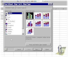
Figure 4.4

Step 4.06 Close the office assistant.

The left scroll box of the chart wizard shows you the chart types that are available. By default this will be set to Column. The right side of the wizard displays the chart sub-types that are available.

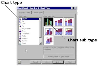
Figure 4.5

Step 4.07 Note how the stage number is displayed at the top of the wizard as well as a set of control buttons at the bottom. These buttons enable you to progress forward or backward through each stage of the wizard.

Step 4.08 Click on the Line chart type instead.

Note that this will display a new chart sub-type on the right hand side of the chart wizard.

Step 4.09 Click on the middle line chart sub type. This is a stacked chart type, which means the value of product 2 will be stacked (placed on top) onto product 1 giving a total of the 2.

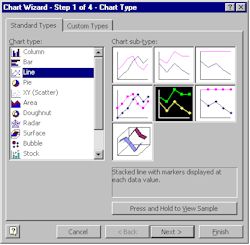
Figure 4.6

Step 4.10 Click on the Next button to take you to stage 2 of the wizard.

Figure 4.7

The chart wizard – Step 2 Chart Source Data
At this step you will specify two things. The first, whether the data range value you initially selected is correct, and secondly, whether you want the chart in row or column format.

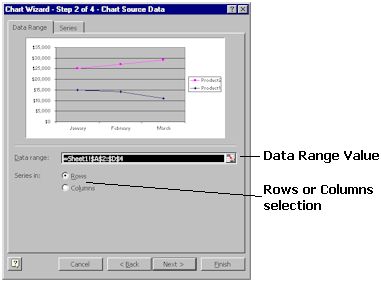
Figure 4.8

Step 4.11 The data range value should read =Sheet1!$A$2:$D$4. If not, highlight the existing value and type in the value listed above.

Step 4.12 By default, the Rows or Columns will be set to Rows so no changes need to be made here.

Step 4.13 Click on the Next button to take you to stage 3 of the wizard.

Figure 4.9

Home | Other Courses | Notes | Feedback